
Why
I’d been down the strange-attractor rabbit hole for a while, with the Lorenz attractor and the chaos game behind me, when I hit the logistic map in Gary William Flake’s The Computational Beauty of Nature. It looked like too much fun not to plot. I wrote it in Python, and the result has been my LinkedIn banner ever since.
The equation
One line of arithmetic:
Read x as a population, scaled to between 0 and 1, and r as its growth rate. For each r, iterate and see where x ends up.
How the plot is made
For every r from 0 to 4, start at x = 0.5 and discard the first 2,000 iterations so the transient dies out. Then keep iterating and record each value until the orbit returns to where it started. If it settles into a cycle, that records exactly one cycle. If it never settles, it records up to 1,001 points. Plot all of them against r.
Reading it
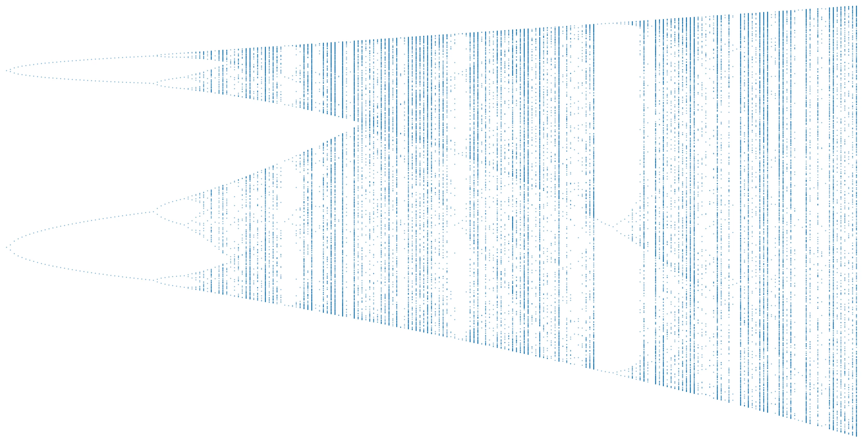
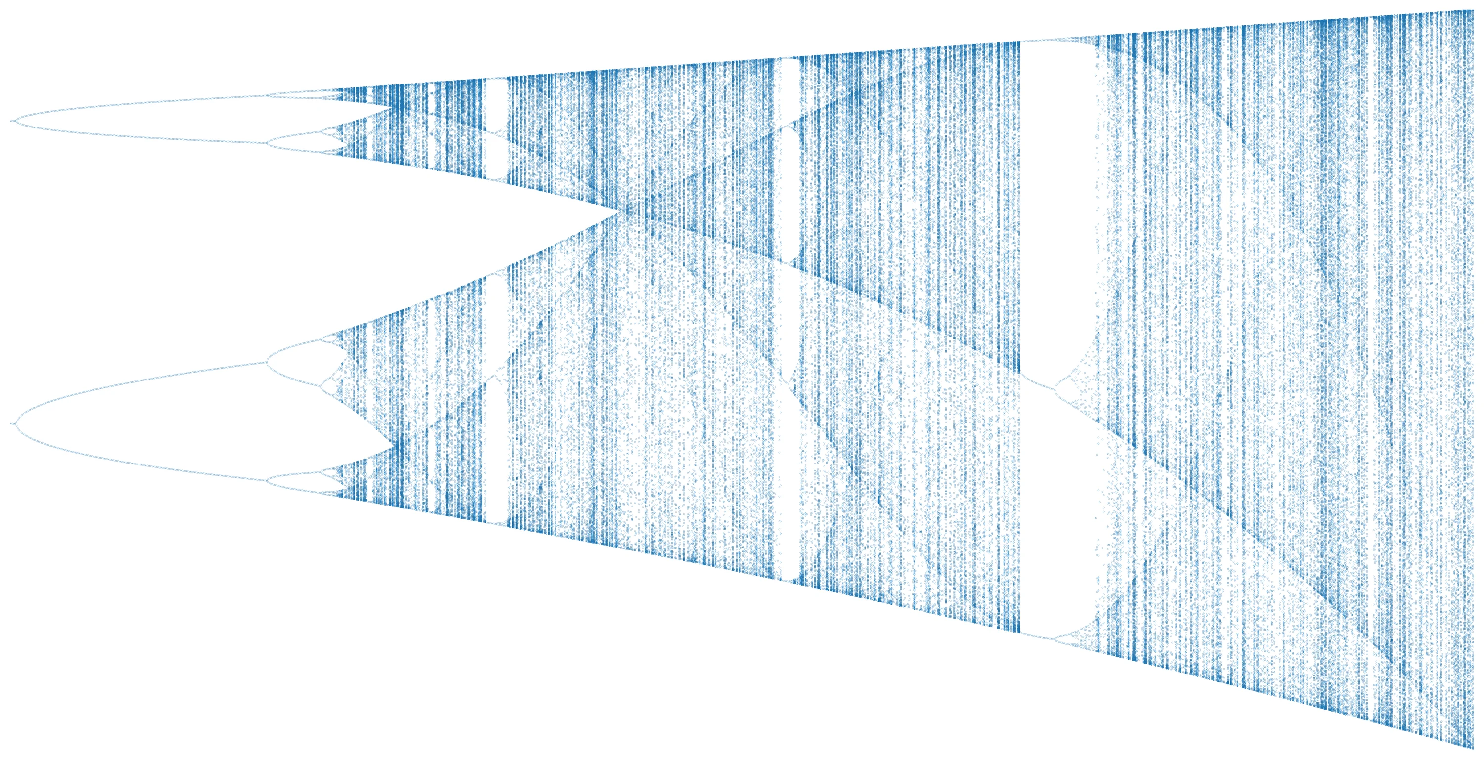
Below r = 3 the population settles to a single value. At r = 3 it splits into two and starts oscillating between them, then four at about 3.449, then eight at about 3.544. The doublings come faster and faster, and past about 3.57 the orderly branches dissolve into chaos. Even inside the chaos there are windows of order. The clear vertical gap near 3.83 is a stable 3-cycle, which shows up out of nowhere.
Shrinking the step in r from 0.0025 to 0.00005 brings out finer and finer structure. The repo has all three renders.
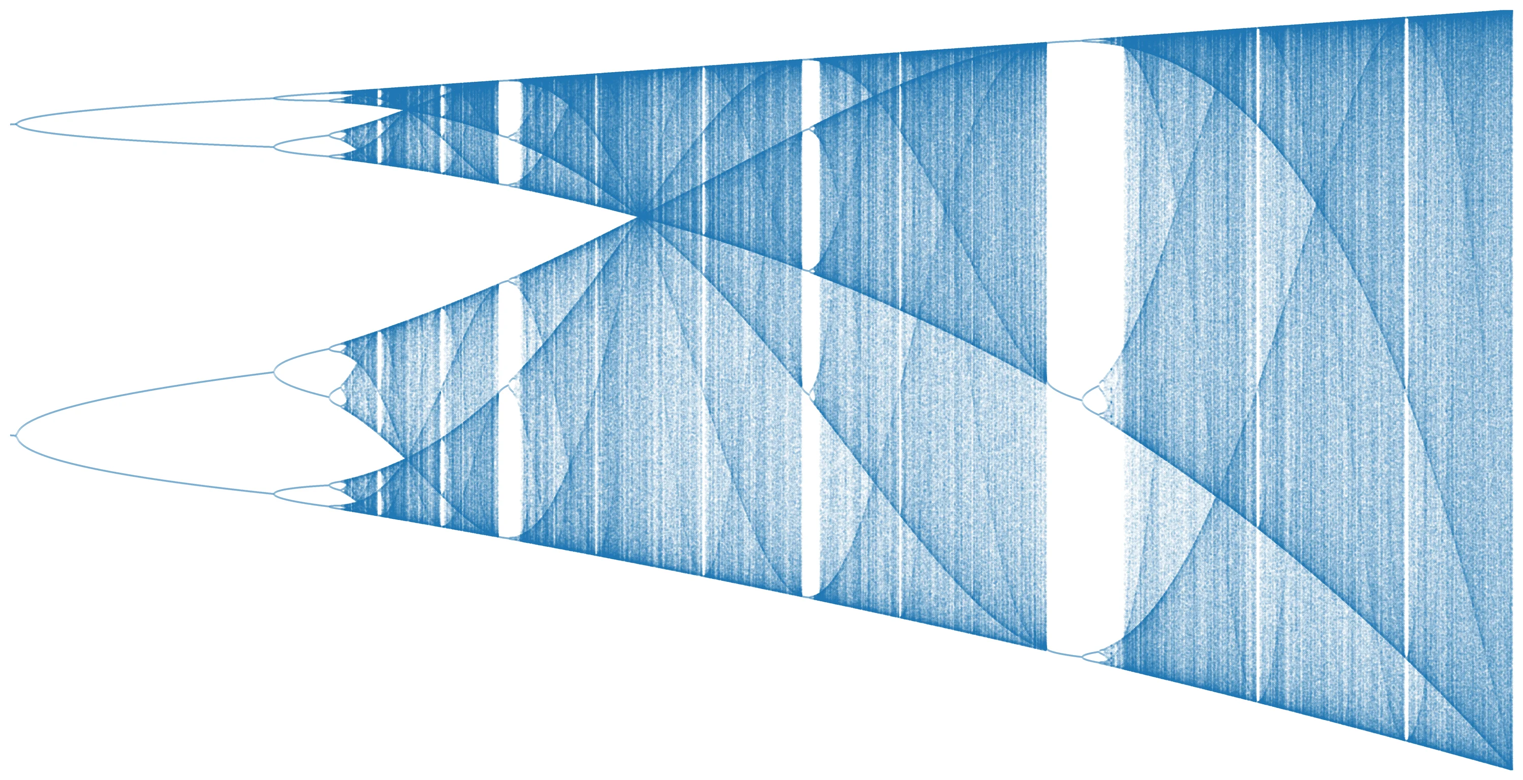
This plot also turns up in A reminder of change, constancy and chaos. I’d been working on it just before writing that post, and it felt right to include it.